spSVC refines the reconstruction of Visium HD profiles and recovers spatial transcriptional patterns at single-cell resolution
Notebook Guide
Purpose. Analyze the Visium HD sp-SVC case using precomputed sp-SVC inputs placed at the original notebook paths.
Inputs. ../../raw_data/Real_application/P1CRC_HD.h5ad, adata_sc_all_reanno.h5ad, and ../../output/sp_SVC_case/P1CRC/sp_SVC.h5ad.
Outputs. Metric comparisons, spatial autocorrelation plots, clustering maps, and marker dot plots displayed inline and saved under ../../output/sp_SVC_case/.
Reading order.
Verify required inputs and cached metrics
Compare original and sp-SVC clustering metrics
Compare spatial autocorrelation
Visualize marker programs in raw and sp-SVC data
Reproducibility note. revise imports are standard package imports from the installed revise-svc distribution; this notebook does not modify sys.path to import the repository source tree.
First glimpse at raw data
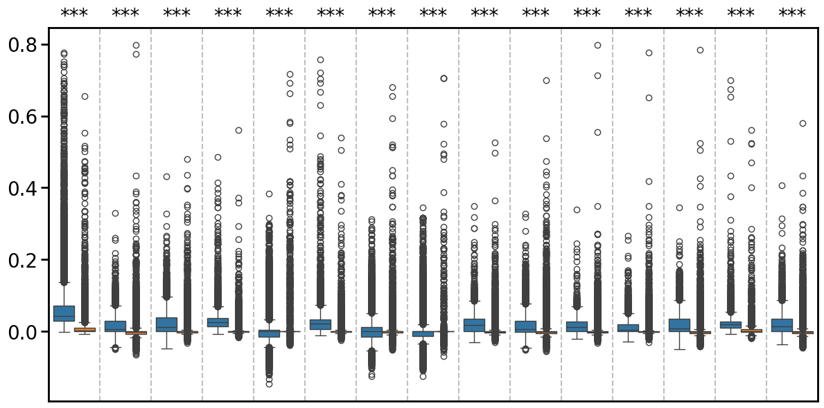
Spatial Autocorrelation
Compare Moran-style spatial autocorrelation summaries between raw and sp-SVC outputs.
[1]:
import os
os.environ.setdefault("TQDM_DISABLE", "1")
os.environ.setdefault("TQDM_MININTERVAL", "60")

try:
    from IPython import get_ipython
    _ipython = get_ipython()
    if _ipython is not None:
        _ipython.run_line_magic("matplotlib", "inline")
except Exception:
    pass

import os

import scanpy as sc
import pandas as pd
import numpy as np

from tqdm import tqdm as _tqdm

def tqdm(iterable=None, *args, **kwargs):
    kwargs.setdefault("disable", True)
    return _tqdm(iterable, *args, **kwargs)
from revise.analysis.spatial_metric import spatial_gene_autocorr, plot_compare_spatial_autocorr, get_sampeled_adata, run_cluster_plot
/cpfs01/projects-HDD/cfff-c7cd658afc74_HDD/jiaoyifeng/miniconda3/envs/brainbeacon/lib/python3.9/site-packages/numba/core/decorators.py:246: RuntimeWarning: nopython is set for njit and is ignored
  warnings.warn('nopython is set for njit and is ignored', RuntimeWarning)
Prerequisites
Before running this analysis notebook, please prepare the following data:
1. Raw Data
Download all raw data from Zenodo
Place the downloaded files in the
[raw_data_path]directory
2. Reconstructed Data (Choose one option)
Option A: Generate locally
Run the script:
application_sc_SVC_recon.sh
Option B: Download pre-computed results
Download all reconstructed data from Zenodo
Place the downloaded files in the
[svc_data_path]directory
[2]:
patient_id = "P1CRC"
data_type = "HD"

raw_data_path = "../../raw_data/Real_application"

raw_file_name = f"{raw_data_path}/{patient_id}_{data_type}.h5ad"
sc_file_name = f"{raw_data_path}/adata_sc_all_reanno.h5ad"
[3]:
adata = sc.read(raw_file_name)
adata.obs['Level1'].value_counts()
[3]:
Level1
Tumor                    142181
Fibroblast               105946
Intestinal Epithelial     64679
SMC                       39477
Mono/Macro                38281
Plasma                    31027
Vascular EC               18013
DC                        15576
T                         14571
B                         11663
Pericyte                  10927
Lymphatic EC               4802
Gliacyte                   4416
Mast                       3756
Unknown                    2369
Name: count, dtype: int64
Clustering metric
[4]:
resolutions = [0.3, 0.5, 0.8]
patient_ids = ["P1CRC"] # one tumor sample for test
patient_ids = ["P1CRC", "P2CRC", "P5CRC"]
patient_ids = ["P1CRC"] # available HD input in this reproducibility environment


data_type = "HD"
cell_type_col = "Level1"

sample_size = 30000

raw_data_path = "../../raw_data/Real_application"
svc_data_path = "../../output/sp_SVC_case"

save_dir = "results/sp_SVC_case"
save_dir = "../../output/sp_SVC_case"
Input And Cache Checks
Confirm that the original relative data paths resolve before running analysis cells.
[5]:
expected_result_suffixes = [
    "original/metric.csv",
    "original/moran_autocorr.csv",
    "sp_SVC/metric.csv",
    "sp_SVC/moran_autocorr.csv",
]

for patient_id in tqdm(patient_ids, desc="Processing patients"):

    save_path = f"{save_dir}/{patient_id}_{data_type}"
    os.makedirs(save_path, exist_ok=True)
    expected_result_files = [f"{save_path}/{suffix}" for suffix in expected_result_suffixes]
    if all(os.path.exists(path) for path in expected_result_files):
        print(f"Using cached core result files for {patient_id}_{data_type}")
        continue

    print(f"Processing original data for {patient_id}_{data_type}")
    adata_sp = sc.read(f"{raw_data_path}/{patient_id}_{data_type}.h5ad")
    adata_sp = adata_sp[adata_sp.obs[cell_type_col] != "Unknown"].copy()

    if sample_size is not None:
        adata_sp = get_sampeled_adata(adata_sp, sample_size=sample_size, seed=0)
        # print(adata_sp.obs[cell_type_col].value_counts())

    run_cluster_plot(adata_sp, f"{save_path}/original",
                        resolutions = resolutions,
                        cell_type_col = "Level1")
    all_sp, select_sp = spatial_gene_autocorr(adata_sp, cell_type_col = "Level1", save_dir = f"{save_path}/original")


    print(f"Processing SVC data for {patient_id}_{data_type}")
    adata_sp_svc = sc.read(f"{svc_data_path}/{patient_id}/sp_SVC.h5ad")

    adata_sp_svc = adata_sp_svc[adata_sp_svc.obs[cell_type_col]!= "Unknown"].copy()

    if sample_size is not None:
        adata_sp_svc = get_sampeled_adata(adata_sp_svc, sample_size=sample_size, seed=0)
        print(adata_sp.obs[cell_type_col].value_counts())

    run_cluster_plot(adata_sp_svc, f"{save_path}/sp_SVC",
                        resolutions = resolutions,
                        cell_type_col = "Level1")
    all_sp_svc, select_sp_svc = spatial_gene_autocorr(adata_sp_svc,
                                                cell_type_col = "Level1",
                                            save_dir = f"{save_path}/sp_SVC",
                                                                )

    plot_compare_spatial_autocorr(all_sp_svc, all_sp, save_dir = save_path, mode = "moran")
Using cached core result files for P1CRC_HD
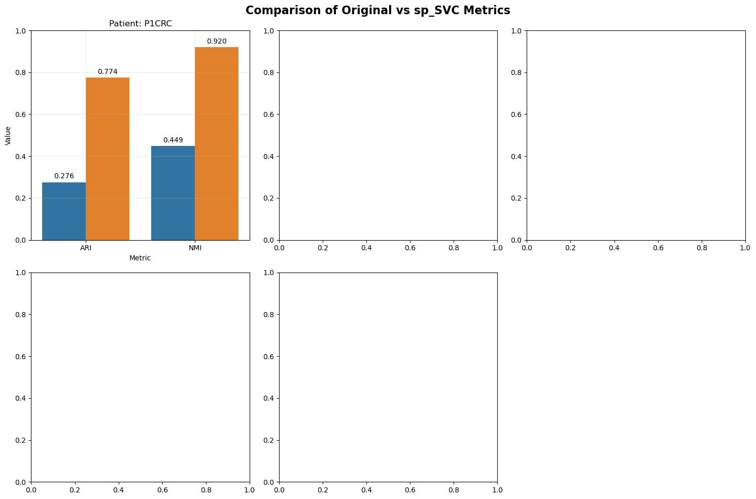
Plot summary ARI and NMI
Metric Comparison
Compare clustering and reconstruction metrics between original and sp-SVC data.
[6]:
import pandas as pd

from tqdm import tqdm as _tqdm

def tqdm(iterable=None, *args, **kwargs):
    kwargs.setdefault("disable", True)
    return _tqdm(iterable, *args, **kwargs)

patient_ids = ["P1CRC"]
metrics = ["ARI", "NMI"]
data_type = "HD"
cell_type_col = "Level1"
[7]:
all_metric_dfs = []

for patient_id in tqdm(patient_ids):
    original_metric_df = pd.read_csv(f"../../output/sp_SVC_case/{patient_id}_{data_type}/original/metric.csv")
    select_res = original_metric_df.loc[original_metric_df['ARI'].idxmax(), "resolution"]
    print(patient_id, select_res)

    original_metric_df = original_metric_df[original_metric_df['resolution'] == select_res]
    original_metric_df['data_class'] = "Original"

    sp_SVC_metric_df = pd.read_csv(f"../../output/sp_SVC_case/{patient_id}_{data_type}/sp_SVC/metric.csv")
    sp_SVC_metric_df = sp_SVC_metric_df[sp_SVC_metric_df['resolution'] == select_res]
    sp_SVC_metric_df['data_class'] = "sp_SVC"

    metric_df = pd.concat([original_metric_df, sp_SVC_metric_df], axis=0)
    metric_df['patient_id'] = patient_id

    all_metric_dfs.append(metric_df)

final_metric_df = pd.concat(all_metric_dfs, axis=0)
P1CRC 0.5
[8]:
import matplotlib.pyplot as plt
import seaborn as sns

fig, axes = plt.subplots(2, 3, figsize=(15, 10))
fig.suptitle('Comparison of Original vs sp_SVC Metrics', fontsize=16, fontweight='bold')

axes = axes.flatten()

for i, patient_id in enumerate(patient_ids):
    patient_data = final_metric_df[final_metric_df['patient_id'] == patient_id]

    plot_data = []
    for metric in metrics:
        for data_class in ["Original", "sp_SVC"]:
            value = patient_data[patient_data['data_class'] == data_class][metric].values[0]
            plot_data.append({
                'Metric': metric,
                'Value': value,
                'Data Class': data_class
            })

    plot_df = pd.DataFrame(plot_data)

    ax = axes[i]
    bars = sns.barplot(data=plot_df, x='Metric', y='Value', hue='Data Class', ax=ax, legend=False)
    ax.set_title(f'Patient: {patient_id}')
    ax.set_ylim(0, 1)
    ax.grid(True, alpha=0.3)

    for container in bars.containers:
        bars.bar_label(container, fmt='%.3f', padding=3)

# Add the legend in the last position (the sixth subplot)
axes[5].set_visible(False)  # Hide the axes of the sixth subplot

plt.tight_layout()
plt.subplots_adjust(top=0.93)  # Leave space for the overall title

plt.savefig(f'{save_dir}/metrics_comparison.pdf', dpi=300, bbox_inches='tight')
plt.show()
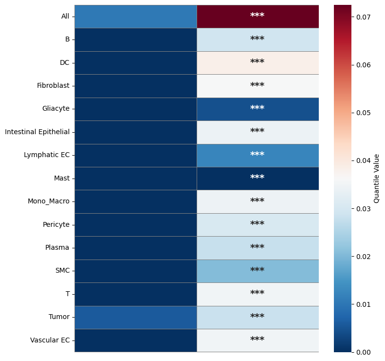
Plot spatial correlation
Heatmap of the moran’I metric in mean or quantile
[9]:
import pandas as pd
import numpy as np

import seaborn as sns
from matplotlib import pyplot as plt
from scipy.stats import ttest_ind
from tqdm import tqdm as _tqdm

def tqdm(iterable=None, *args, **kwargs):
    kwargs.setdefault("disable", True)
    return _tqdm(iterable, *args, **kwargs)

def plot_compare_spatial_autocorr_heatmap(df_sp_svc, df_original, save_dir, mode="moran",
                                         statistic="mean", quantile=0.5, cmap="viridis"):
    """
    Generate a heatmap comparing two dataframes across cell types with significance testing.

    Parameters:
    df_sp_svc (pd.DataFrame): Dataframe with genes as rows, cell types as columns.
    df_original (pd.DataFrame): Dataframe with genes as rows, cell types as columns.
    save_dir (str): Directory to save the heatmap image.
    mode (str): Mode identifier for the output filename.
    statistic (str): Statistic to calculate - "mean" or "quantile".
    quantile (float): Quantile to calculate if statistic is "quantile" (0-1).
    cmap (str): Colormap for the heatmap.
    """

    # Prepare data for heatmap
    cell_types = df_sp_svc.columns.intersection(df_original.columns)

    # Calculate statistics and p-values
    stats_data = []
    p_values = []

    for cell_type in cell_types:
        # Extract values for each cell type
        sp_svc_values = df_sp_svc[cell_type].dropna()
        original_values = df_original[cell_type].dropna()

        # Calculate selected statistic
        if statistic == "mean":
            sp_svc_stat = sp_svc_values.mean()
            original_stat = original_values.mean()
        elif statistic == "quantile":
            sp_svc_stat = sp_svc_values.quantile(quantile)
            original_stat = original_values.quantile(quantile)
        else:
            raise ValueError("statistic must be 'mean' or 'quantile'")

        # Calculate p-value
        if len(sp_svc_values) > 1 and len(original_values) > 1:
            _, p_val = ttest_ind(sp_svc_values, original_values, nan_policy='omit')
        else:
            p_val = 1.0  # Not enough data for test

        stats_data.append([original_stat, sp_svc_stat])
        p_values.append(p_val)

    # Create dataframe for heatmap
    heatmap_df = pd.DataFrame(stats_data,
                             index=cell_types,
                             columns=['Original', 'SP_SVC'])

    # Create annotation matrix with significance stars
    annotation_matrix = []
    for p_val in p_values:
        if p_val < 0.05:
            sig = '*' if p_val >= 0.01 else '**' if p_val >= 0.001 else '***'
            annotation_matrix.append(['', sig])
        else:
            annotation_matrix.append(['', ''])

    # Create the heatmap
    plt.figure(figsize=(8, max(6, len(cell_types) * 0.5)))

    # Plot heatmap with specified colormap
    sns.heatmap(heatmap_df,
                annot=np.array(annotation_matrix),  # Use annotations for significance
                fmt='',  # Empty format since we're using custom annotations
                cmap=cmap,
                cbar_kws={'label': f'{statistic.capitalize()} Value'},
                linewidths=0.5,
                linecolor='gray',
                # vmin=-0.01,
                # vmax=0.1,
                annot_kws={'fontsize': 14, 'fontweight': 'bold'})

    plt.ylabel('')
    plt.xlabel('')
    plt.xticks([])

    # Adjust layout and save
    plt.tight_layout()
    plt.savefig(f"{save_dir}/Compare_{mode}_{statistic}_heatmap.pdf", dpi=300, bbox_inches='tight')
    plt.show()
    plt.close()
[10]:
data_type = "HD"
mode = "moran"
patient_ids = ["P1CRC"]

save_dir = f"../../output/sp_SVC_case/{patient_id}_{data_type}"
for patient_id in tqdm(patient_ids, desc = "patient_id"):

    moranI_sp_file = f"{save_dir}/original/{mode}_autocorr.csv"
    moranI_sp = pd.read_csv(moranI_sp_file, index_col = 0)
    moranI_sp.columns = moranI_sp.columns.str.replace("/", "_")
    # moranI_sp
    moranI_sp_svc_file = f"{save_dir}/sp_SVC/{mode}_autocorr.csv"
    moranI_sp_svc = pd.read_csv(moranI_sp_svc_file, index_col = 0)
    # moranI_sp_svc

    plot_compare_spatial_autocorr_heatmap(moranI_sp_svc, moranI_sp, save_dir, mode="moran",
                                         statistic="quantile", quantile=0.75, cmap="RdBu_r")
Boxplot of the moran’I metric
[11]:
import pandas as pd
import seaborn as sns
from matplotlib import pyplot as plt
from tqdm import tqdm as _tqdm

def tqdm(iterable=None, *args, **kwargs):
    kwargs.setdefault("disable", True)
    return _tqdm(iterable, *args, **kwargs)
from scipy.stats import ttest_ind

def plot_compare_spatial_autocorr(df_sp_svc, df_original, save_dir, mode = "moran"):
    """
    Generate a boxplot comparing two dataframes across cell types with significance testing.

    Parameters:
    df_sp_svc (pd.DataFrame): Dataframe with genes as rows, cell types as columns.
    df_original (pd.DataFrame): Dataframe with genes as rows, cell types as columns.
    output_file (str): Path to save the boxplot image.
    """

    # Prepare data for boxplot
    cell_types = df_sp_svc.columns.intersection(df_original.columns)
    data = []
    for cell_type in cell_types:
        # Extract values for each cell type
        sp_svc_values = df_sp_svc[cell_type].dropna()
        original_values = df_original[cell_type].dropna()
        # Add to data list with labels
        for val in sp_svc_values:
            data.append({'Cell Type': cell_type, 'Value': val, 'Source': 'SP_SVC'})
        for val in original_values:
            data.append({'Cell Type': cell_type, 'Value': val, 'Source': 'Original'})

    # Convert to dataframe
    plot_df = pd.DataFrame(data)

    # Set up the boxplot
    plt.figure(figsize=(12, 6))
    plot_df = plot_df[plot_df["Value"] < 0.8]
    sns.boxplot(x='Cell Type', y='Value',
                hue='Source', data=plot_df,
                palette=['#1f77b4', '#ff7f0e'],
                legend=False)


    # Add dashed lines between cell types
    for i in range(len(cell_types) - 1):
        plt.axvline(x=i + 0.5, color='gray', linestyle='--', alpha=0.5)

    # Rotate x-axis labels
    plt.xticks(rotation=30, ha='right')

    # Add significance annotations
    for i, cell_type in enumerate(cell_types):
        sp_svc_vals = plot_df[(plot_df['Cell Type'] == cell_type) & (plot_df['Source'] == 'SP_SVC')]['Value']
        orig_vals = plot_df[(plot_df['Cell Type'] == cell_type) & (plot_df['Source'] == 'Original')]['Value']
        if len(sp_svc_vals) > 0 and len(orig_vals) > 0:
            t_stat, p_val = ttest_ind(sp_svc_vals, orig_vals, nan_policy='omit')
            # Add stars for significance
            if p_val < 0.05:
                sig = '*' if p_val >= 0.01 else '**' if p_val >= 0.001 else '***'
                max_y = max(sp_svc_vals.max(), orig_vals.max())
                text_y = max_y + 0.05 * (plot_df['Value'].max() - plot_df['Value'].min())
                text_y = 0.85
                plt.text(i, text_y,
                        sig, ha='center', va='bottom', fontsize=20)

    # Adjust layout and save
    plt.xlabel('')
    plt.ylabel('')
    plt.xticks([])
    plt.yticks(fontsize = 20)

    # Get the current Axes object
    ax = plt.gca()
    # Set the outer border line width
    for spine in ax.spines.values():
        spine.set_linewidth(2)

    ax.tick_params(axis='y', which='major', width=2, length = 8)

    plt.tight_layout()
    plt.savefig(f"{save_dir}/Compare_{mode}.png")
    plt.show()
[12]:
data_type = "HD"
mode = "moran"
patient_ids = ["P1CRC"]

save_dir = f"../../output/sp_SVC_case/{patient_id}_{data_type}"

for patient_id in tqdm(patient_ids, desc = "patient_id"):

    moranI_sp_file = f"{save_dir}/original/{mode}_autocorr.csv"
    moranI_sp = pd.read_csv(moranI_sp_file, index_col = 0)
    moranI_sp.columns = moranI_sp.columns.str.replace("/", "_")
    # moranI_sp
    moranI_sp_svc_file = f"{save_dir}/sp_SVC/{mode}_autocorr.csv"
    moranI_sp_svc = pd.read_csv(moranI_sp_svc_file, index_col = 0)
    # moranI_sp_svc

    plot_compare_spatial_autocorr(moranI_sp_svc, moranI_sp, save_dir = save_dir, mode = "moran")
Analysis CAF surrounded tumor in P1CRC
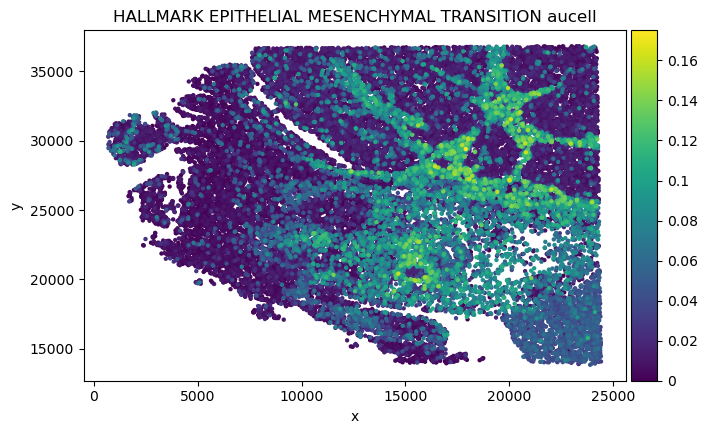
sp-SVC recovers spatially organized EMT-associated transcriptional programs and identifies genes linked to clinical significance
[13]:
import scanpy as sc
from revise.analysis.spatial_metric import preprocess_adata

raw_data_path = "../../raw_data/Real_application"
svc_data_path = "../../output/sp_SVC_case"

patient_id = "P1CRC"
data_type = "HD"

raw_file_name = f"{raw_data_path}/{patient_id}_{data_type}.h5ad"
sp_SVC_file_name = f"{svc_data_path}/{patient_id}/sp_SVC.h5ad"
adata_sp = sc.read_h5ad(raw_file_name)
adata_sp_svc = sc.read_h5ad(sp_SVC_file_name)
Pathway: EMT (Epithelial-Mesenchymal Transition)
Download Gene Set
Download the “H: hallmark gene sets” GMT file from GSEA MSigDB
Setup Directory
Create a directory named
[pathway]Move the downloaded GMT file into this directory
[14]:
from revise.analysis.spatial_metric import read_gmt, get_sampeled_adata

gmt_file_path = './pathway/h.all.v2025.1.Hs.symbols.gmt'
pathway_dict = read_gmt(gmt_file_path)
print(len(pathway_dict))

select_sp_svc = get_sampeled_adata(adata_sp_svc, sample_size = 30000, seed = 42)
50
Sampling 30000 cells from 424433 total cells.
[15]:
from revise.analysis.spatial_metric import get_pathway_score, plot_pathway

pathway_name = 'HALLMARK_EPITHELIAL_MESENCHYMAL_TRANSITION'
pathway_dict = {pathway_name: pathway_dict[pathway_name]} # filter

score_method = "AUC"
save_dir = f"../../output/sp_SVC_case/{patient_id}_{data_type}"
[16]:
plot_pathway(select_sp_svc, pathway_dict, score_method,
                save_dir = f"{save_dir}/sp_SVC",
                save_file_format = "png")
189 200
ctxcore have been install version: 0.2.0
<Figure size 1200x1000 with 0 Axes>
<Figure size 640x480 with 0 Axes>
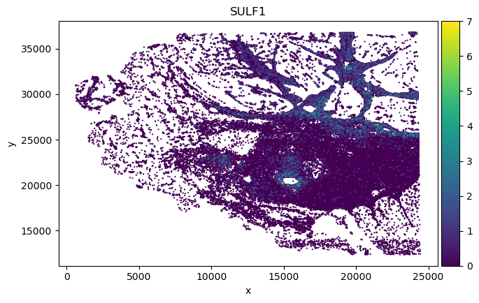
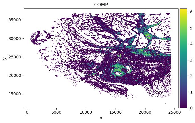
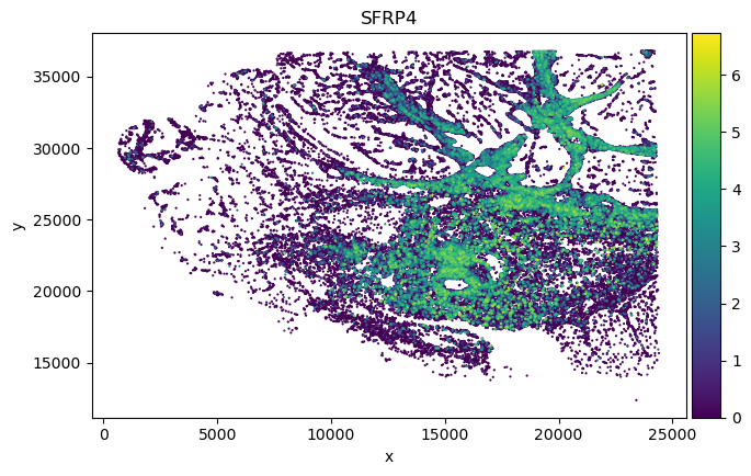
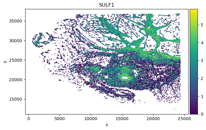
We found in Fibroblast, gene COMP, SFRP4 and SULF1 show high correlation with EMT pathway score.
[17]:
genes = ["COMP", "SFRP4", "SULF1"]

select_ct = "Fibroblast"
adata_sp = adata_sp[adata_sp.obs["Level1"] == select_ct]

adata_sp_svc = adata_sp_svc[adata_sp_svc.obs["Level1"] == select_ct]
adata_sp_svc = preprocess_adata(adata_sp_svc)
[18]:
cmap = "Reds"
cmap = None
size = 10
[19]:
adata_sp_genes = adata_sp[:, genes]
adata_sp_svc_genes = adata_sp_svc[:, genes]

print("Original adata gene spatial expression:")
for gene in genes:
    sc.pl.scatter(adata_sp_genes, x="x", y="y",
                  color=gene,
                  size=size,
                  color_map=cmap,
                  )
print("sp_SVC adata gene spatial expression:")
for gene in genes:
    sc.pl.scatter(adata_sp_svc_genes, x="x", y="y",
                  color=gene,
                  size=size,
                  color_map=cmap,
                  )
Original adata gene spatial expression:
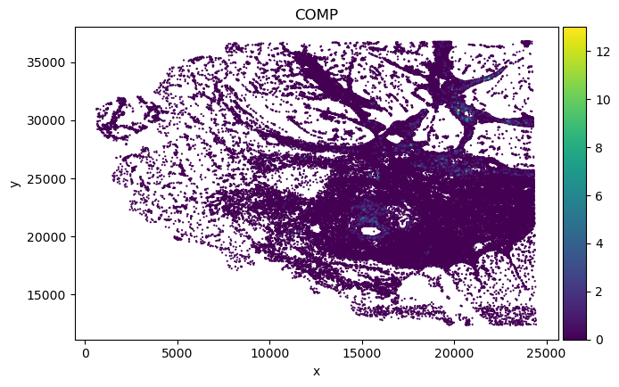
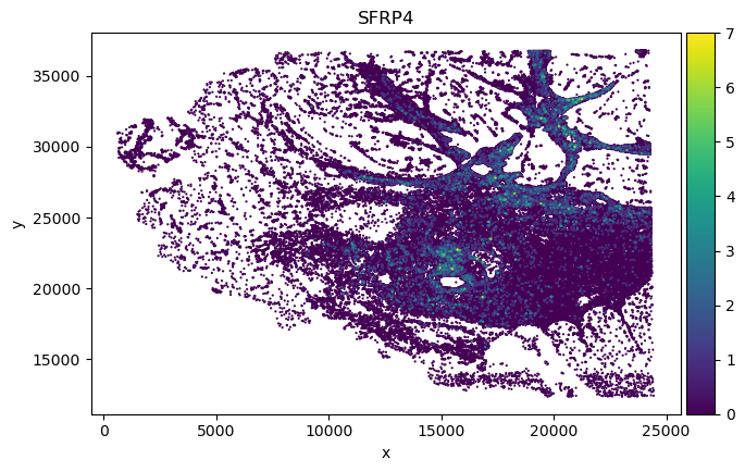
sp_SVC adata gene spatial expression:
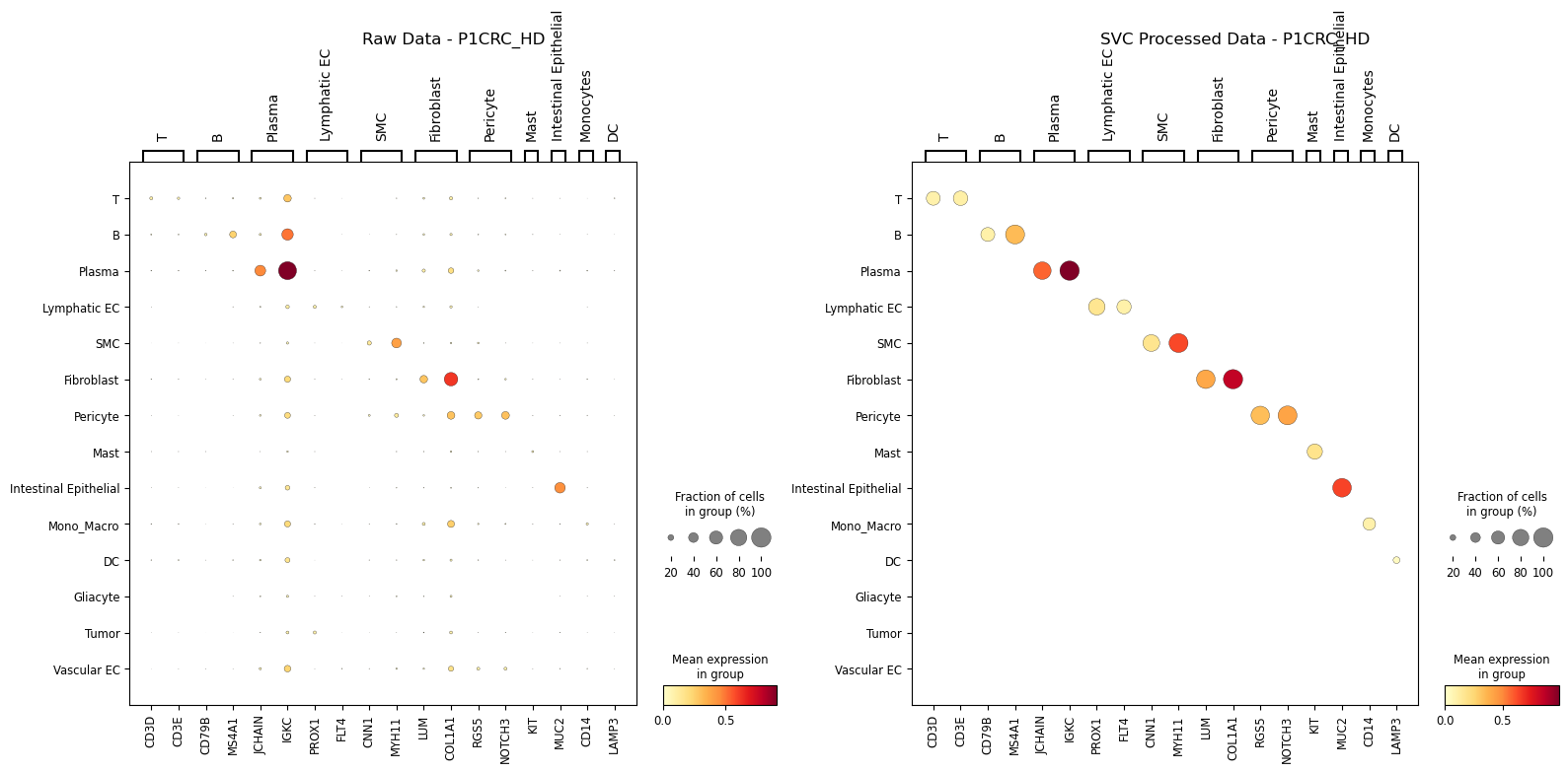
Dotplot analysis to visualize marker specificity
[20]:
import scanpy as sc
from revise.analysis.spatial_metric import preprocess_adata

raw_data_path = "../../raw_data/Real_application"
svc_data_path = "../../output/sp_SVC_case"

patient_id = "P1CRC"
data_type = "HD"

raw_file_name = f"{raw_data_path}/{patient_id}_{data_type}.h5ad"
sp_SVC_file_name = f"{svc_data_path}/{patient_id}/sp_SVC.h5ad"
adata_sp = sc.read_h5ad(raw_file_name)
adata_sp_svc = sc.read_h5ad(sp_SVC_file_name)
[21]:
from revise.analysis.spatial_metric import get_sampeled_adata

adata_sp = get_sampeled_adata(adata_sp, sample_size = 30000, seed = 42)
adata_sp_svc = get_sampeled_adata(adata_sp_svc, sample_size = 30000, seed = 42)
Sampling 30000 cells from 507684 total cells.
Sampling 30000 cells from 424433 total cells.
[22]:
gene_list = [
    # T cells
    "CD3D", "CD3E", "CD2", "TRAC", "TRBC1", "CD4", "CD8A", "CD8B", "IL7R",
    # B cells
    "MS4A1", "CD19", "CD79A", "CD79B", "PAX5",
    # Plasma cells
    "MZB1", "JCHAIN", "XBP1", "PRDM1", "IGKC",
    # NK cells
    "KLRD1", "NKG7", "GNLY", "PRF1", "GZMB", "GZMA",
    # Monocytes
    "CD14", "FCGR3A", "S100A8", "S100A9", "LYZ",
    # Macrophages
    "CD68", "CD163", "MARCO", "MRC1", "MSR1",
    # Dendritic cells
    "CLEC9A", "ITGAX", "CD1C", "LAMP3", "IRF8",
    # Mast cells
    "TPSAB1", "TPSB2", "KIT", "CMA1",
    # Vascular endothelial
    "PECAM1", "VWF", "CDH5", "KDR", "CLDN5",
    # Lymphatic endothelial
    "PROX1", "LYVE1", "PDPN", "FLT4",
    # Fibroblasts
    "COL1A1", "COL1A2", "COL3A1", "DCN", "LUM", "FAP", "PDGFRA",
    # Pericytes
    "RGS5", "PDGFRB", "CSPG4", "ACTA2",
    # Smooth muscle cells
    "ACTA2", "TAGLN", "MYH11", "CNN1",
    # Intestinal epithelial
    "EPCAM", "KRT19", "KRT8", "MUC2", "TFF3", "CDH1",
    # Tumor cells (general)
    "EPCAM", "KRT18", "KRT8", "MKI67", "SOX2"
]
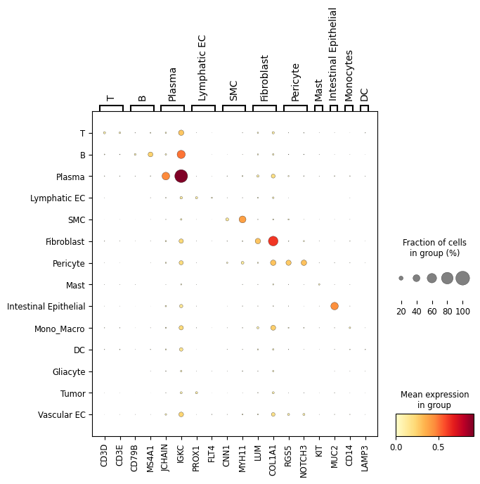
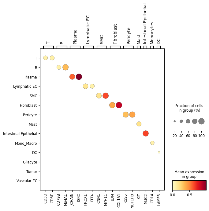
Marker Program Visualization
Show marker-gene dot plots for raw and sp-SVC expression layers.
[23]:
selected_marker_genes = {
    # 'T': [ "CD2", "TRBC1",],
    'T': [ "CD3D", "CD3E",],
    'B': [ "CD79B", "MS4A1"],
    'Plasma': ["JCHAIN", "IGKC"],
    'Lymphatic EC': ["PROX1", "FLT4"],
    'SMC': ["CNN1","MYH11"],
    'Fibroblast': [ "LUM", "COL1A1"],
    'Pericyte': ["RGS5", "NOTCH3"],
    'Mast': ["KIT"],
    'Intestinal Epithelial': ["MUC2"],
    'Monocytes': ["CD14"],
    'DC': ["LAMP3",],
}
[24]:
def add_cutoff_layer(adata, cutoff = 2):
    adata.layers['cutoff'] = adata.X.copy()
    adata.layers['cutoff'][adata.layers['cutoff'] > cutoff] = cutoff

    return adata
[25]:
cutoff = 1
adata_sp = add_cutoff_layer(adata_sp, cutoff=cutoff)
adata_sp_svc = add_cutoff_layer(adata_sp_svc, cutoff=cutoff)
[26]:
desired_order = ['T', 'B', 'Plasma', 'Lymphatic EC',
                 'SMC', 'Fibroblast', 'Pericyte',
                  'Mast',
                  'Intestinal Epithelial','Mono_Macro','DC',
                'Gliacyte',  'Tumor','Vascular EC',
     ]
adata_sp.obs['Level1'].replace('Mono/Macro', 'Mono_Macro', inplace=True)
adata_sp = adata_sp[adata_sp.obs['Level1'].isin(desired_order)]
adata_sp.obs['Level1'] = adata_sp.obs['Level1'].cat.reorder_categories(desired_order)

adata_sp_svc = adata_sp_svc[adata_sp_svc.obs['Level1'].isin(desired_order)]
adata_sp_svc.obs['Level1'] = adata_sp_svc.obs['Level1'].cat.reorder_categories(desired_order)
[27]:
import matplotlib.pyplot as plt

groupby = "Level1"
fig, (ax1, ax2) = plt.subplots(1, 2, figsize=(16, 8))


cmap = 'YlOrRd'

sc.pl.dotplot(adata_sp, selected_marker_genes, groupby,
              layer="cutoff",
              dendrogram=False, ax=ax1, show=False,
              cmap=cmap)
ax1.set_title(f'Raw Data - {patient_id}_{data_type}')

sc.pl.dotplot(adata_sp_svc, selected_marker_genes, groupby,
              layer="cutoff",
              dendrogram=False, ax=ax2, show=False,
              cmap=cmap)
ax2.set_title(f'SVC Processed Data - {patient_id}_{data_type}')

plt.tight_layout()
plt.show()
[28]:
# save
save_dir = '../../output/sp_SVC_case'
cmap = 'YlOrRd'


# plt.figure(figsize=(10, 6))
sc.pl.dotplot(adata_sp, selected_marker_genes, groupby,
              layer="cutoff",
              dendrogram=False, show = False,
              cmap = cmap,
              figsize=(7, 6)
              )
plt.savefig(f"{save_dir}/{patient_id}_{data_type}/raw_dotplot.pdf")
plt.show()
plt.close()

# plt.figure(figsize=(10, 6))
sc.pl.dotplot(adata_sp_svc, selected_marker_genes, groupby,
              layer="cutoff",
              dendrogram=False, show = False,
              cmap = cmap,
              figsize=(7, 6)
              )
plt.savefig(f"{save_dir}/{patient_id}_{data_type}/svc_dotplot.pdf")
plt.show()
plt.close()